How to Draw a Line Between Two Points on Desmos

Actions

An action is an instruction ( or a list of instructions ) that can be run when you want.
The implicit syntax is a→1 to set a = 1 when the action will be triggered. a→b, b→a for a series of instructions (note that the actions on a and b are simultaneous, so no need of an intermediate variable to swap values).
The explicit form is S = a→1 to name this action for later use.
From here, you can click on the arrow in the margin to trigger the action.

e.g.:

S = { i<10: i→i+1} : increment at each triggering, up to 10
S = a→ { a=0: 1, 0 } : flip-flops the value of a at each triggering of S.
S = i→i+1, L→join(L,f(i)) : piles up a new value of f() in the list L
Attention: done many many times, this may generate ultra long lists, up to freezing your machine. Take care to secure a limit (e.g., join only as i<100 ).

if necessary, S can even have parameters: S(v) = a→ v

Important note:
For some unknown reason, for now you have first to activate the feature (once and for all) in your account (advanced parameters).

Events

You could already easily get some interaction via sliders. Even off/on effect or selection within a list of parameters or functions could be done (with some effort) via integer sliders. But there is now a more direct way:
All visible objects ( points, curves, etc ) now have a "clickable" field in the parameters menu. In this field you can enter an explicit action ( like i→i+1 ) or just call its name ( e.g. S , above ).

Ticker, for animation

Animation is obtained by automatically triggering an action over time.
Ticker is done for that : click on "Add" to get the ticker ( only one per graph ). Choose a timer delay ( or let 0 if it should run as often as possible ), and provide the explicit or implicit ( or combined list ) of actions to trigger at each tick.

Attention: if ticker modifies a long list, updating the display of the text version in the commands display may slow down the graph by *a huge* factor → put the list in a folder, and close it for the list does not appear in text.

An extra variable dt is available in this field, measuring the time ( in milliseconds) since the previous call.
e.g. fps → round(1000/dt) store the current frames per second performances in variable fps, that you can display with some point label ${fps} .

more information here.
examples: simulations and automata
examples from the old "beta features" section are still working

Desmos provides many accessibility features, includes playing curves as sound: we can use it to encode melodies.
Bottomest vs toppest lines of the graph correspond to the range of an octave, so it's important to accurately frame your grid then avoid scaling and translating the graph. Using numerical grid setting is the most robust way. Then, the 12 steps within this range correspond to the half-tones in the music scale. Of course you may try continuous variations too !

To activate sound playing of curves:

Select a curve
Open the keypad ( bottom-left icon) and click on the audio button.
or Hit Alt-T → it opens a sound bar at bottom
Click "play" or hit H. Note that you can modify some parameters, like speed.

Sliders

Making a movable point from variables respects their constraints.
→ this allows for 1D sliders:
set v=1 , then settle some value range. then draw point (0,v), and makes it vertically movable (in facts it is the default).

Note that DesmosGraph is smart enough so that even translation and scaling are permitted to draw your slider: (0, v/2 + 1/2 ) . ( But not non-linear transforms ).

Same principle to tune 2 variables as a square 2D slider.

What about other shapes, e.g., disk ?
DesmosGraph allows to put equation everywhere, comprising in parameters tunings, so that the second parameter range can be constrained by the first: range -sqrt(1-v²), sqrt(1-v²)

Example here. More extreme: spiral slider.

Keyboard user control

Desmos have multiple input and output alternatives, to help with various disabilities.
One of the features is that many thing can be controlled from the keyboard.
This include selecting a movable point ( use CTRL-ALT-P , then TAB or shift TAB to browse points ) and moving it ( using arrow keys ).
Practical use: to let the user control 1 ot 2 parameters via keyboard, put a discrete movable point somewhere, and just tell users to first do CTRL-ALT-P once, then use arrow keys.

Example here.

Alternate solutions for motion control:

Detect steps in a slider: click on slider, press 4x TAB (blue halo) for keyboard control. Then use left, right, pgdown, pgup. Measuring the step allows to detect the key typed. Keys Home, End could also be detected on the same principle.
Example here (from an idea by copper_tones).

For alphabetic keys:

Predefining lists with the names of the target keys, so that their multiplication produce the effects (e.g. 3D motion ):
go here. Then click on Input ( line 2 ) and type any of the defined keys a,A,s,S,d,D,w,W,i,I,k,K,j,J,l,L

Interrupted contours

Sometime you want to store several contours or shapes in a same list.
This is possible, because DesmosGraph knows special numbers "undefined" like 0/0 , and "infinity", like 1/0 or infty command.
The first can be used to interrupt contours, the second to make horizontal or vertical asymptotes.

Example here.

Function selector

Sometime you want to test a transform other several possible functions, or let the user experiment. Instead of changing the formula for f(x) or swapping the namings f_i(x) vs f(x), you can implement a function selector by storing them in a table: F(x) = [ all functions ] then f(x) = F(x)[s] .
Example here.

Copy-Pasting a Graph in another

Sometime you make ( or find ) utilitary graphs, e.g. with functions for complex, or geometry, or 3D, or Fourier, or music, or whatever. You would like to include them for use in your new shader.
→ in your graph, create a folder, and just copy the URL in the folder name !
( Attention: the utilitary graph must have no folders, though ).

Extending DesmosGraph

Disclaimer: This is the most technical and unreasonable post on this blog. Ephemeral & hazardous stuff here.

There are 3 ways to extend DesmosGraph with more features:

For programmers, the Desmos API lets you use and interact with Desmos elements within your own JS programs. I won't address this here, see Desmos API ( help in the official API googlegroup and in the unofficial "programming" channel in the desmos discord forum ).
Adding plugins. Attention, these are non official, and might break with new versions of DesmosGraph.
Secret beta-features. Attention, these are unpublic and experimental, so they can disappear or change at any time, and have many bugs. Just for fun !

Plugins:

Chrome plugins:
- Desmodder :
  - Paste ASCIIMath (such as the results of Wolfram Alpha queries) into Desmos
  - export videos
  - Press Ctrl+Q to duplicate an expression, and various other shortcuts
  - Find and replace expressions
  - activate advanced modes (see next section)
  - More to come !
- Desmos More Greek Letters : add all missing Greek letters : just type them !
- LaTeX, Desmos, and PDF extension: turn equations and graphs to gif
- for teachers: Desmos Dashboard Download to csv
Firefox plugins:
- Note that you can install (some) chrome plugins using Chrome Store Foxified
- DesmosLoader (?)
Tampermonkey scripts: ( works everywhere: first install Tampermonkey Chrome or Firefox plugin. Greasemonkey, Firemonkey, etc, are often compatible too. )
- Wolfram2Desmos : copy-paste text-math expression to Desmos
- DesModder : pack the above + more. Ancester of the chrome plugin. Attention: don't run both !
- DesmosGallery: Make a web gallery from all your graphs !
- automatic Desmos Settings
- DesmosToSVG : SVG export button
- screenshot capture
- SlimRunner's interface improvements:
  e.g. : ( see url for the other scripts, more specialized )
  - Art tools: add a color picker
  - Table tools: use mouse click to add points in a table

Custom fonts as curves: by converting font files with a script, but simpler to just copy-paste these results.

Secret beta-features

Attention, these are unpublic and experimental, so they can disappear or change at any time, and have many bugs. Just for fun !

Simulation:
[ UPDATE: ] deprecated. The feature is now official, but works differently. See here.
Still, the examples below have been converted.Run equations at every frame of an animation (choose the rate), or just when clicking "1 step".
This open a whole new world of reactive animations, simulations and games !
Principle: name the variable(s) to be updated with the equation(s) you give.
Trick: if you update big arrays, hide them in closed folder for better perfs.
To activate it:
F12 to go to the JS console, then enter Calc.updateSettings({clickableObjects: true}) +return, then F12 to exit.
Active buttons :
[ UPDATE: ] The feature is now official, but works a bit differently. See here.
Still, the examples below have been converted.Run equations each time a point is clicked. To switch on-off something, or so more: e.g. one step of simulation above.
To activate it:
as above. Points will now show a new option: clickable ( only for not movable points ).
But for this one, attention: when people load your graph they do can use the feature, but they won't see the update equations if they don't activate the feature.
Advanced styling:
More styling options for points and lines, before they (maybe) get public. (free colors once where there).
To activate it:
F12 to go to the JS console, then enter Calc.updateSettings({advancedStyling: true}) +return, then F12 to exit.
Secret folders:
Adds a "hide" option to folders. Useful for hiding intermediate details or cumbersome utilitary functions… as well as spoilers, for teachers :-p . Example here.
To activate it:
F12 to go to the JS console, then enter Calc.updateSettings({administerSecretFolders: true}) +return, then F12 to exit.
3D mode:
no longer available.

Examples:
– Interactive drawing (with reset button).
– Conway game of life cellular automata.
– See various simulations and automata in this reddit Desmos competition.

URL + parameter

You can also control the aspect at launch, and activate various secret parameters and features, by adding parameters to the graph URL:

url?param₁&param₂&...param_n

They are all listed and detailed here.

Short card:

Default colors: invertedColors, textColor=FF0000, backgroundColor=DDDDFF
Default mode: projectorMode, lang=<lang>
Desactivate interface elements: lockViewport, nographpaper, nozoomButtons, nokeypad, nosettingsMenu, nobranding, noexpressionsTopbar, embed
Tune secret features: clickableObjects, advancedStyling, timeoutLoop=<simulation/slider ms>
Monitor performances: timeInWorker, simulationFPS

We can use either points (x,y) or arrays [x,y] to implement complex, then redefine all classical operators mul, div, pow, exp, log. ( addition, subtraction, multiplication by scalar works directly ).

Implementation with points
Advantages:
– directly displayable and dragable.
– points can contain lists ( to generate automatically a set of complexes )
Inconvenient: you cannot compare or solve points.

Implementation with arrays
Big advantage: you can compare and solve array: see Inversion below.
Inconvenients:
– you have to convert to/from points for display or drag parameters.
– you cannot have list or list, so you can't generate automatically a set of complexes.

Note that to display the mapping of space via a complex transform we would like to display the transformed grid, via solving f(X) = grid. Alas, only array-complexes allow solving while only points-complexes allow grids. But we can still do that by testing that values are integer via mod()=0, or near integer.

Example: complex inversion

For once this is not about a hidden feature or advanced trick: it is about a not know enough incredibly powerful function of DesmosGraph: fitting, i.e., finding the parameters of a simple target curve best approaching your raw data or your too complex function.
Many tools propose least square method to fit a line on a set, but DesmosGraph is a very rare tool allowing you to fit equations or data to really any shape you like, with any kind of parameters. And this can also be used for multidimensional functions.
And all this ultra simple: complexfunc(X) ~ simplefunc(X) , where simplefunc(x) is defined as usual, with use of free parameters as usual (just don't define them, fitting will). X is an array of values, since fitting work on data sets.

Simple example

2D example

In the definition of g(), you can add contraints on the parameters , e.g. { -1 ≤ b ≤ 1 } to restrict search domain (in some complex situations this can help).

More about the history of this feature, and about advanced advices to handle complex cases here.

New (v 1.6) :

Desmos Graph now have color functions !
var = rgb(r,g,b) (r,g,b in 0..255 ) , orvar = hsv(h,s,v) ( h in 0..360, s and v in 0…1 )

Declaring this add a new color to the palette you can use when choosing colors.
You can use any expression, possibly depending on an existing variable (e.g. time). NB: The variable name is compulsory, despite of no use for you.

A cool use is to define array values for colors: then if you draw an array of points or curves and set this "color" to it, each successive element will use the successive color in the array.
See example1, example2, example3.

desmos-graph (6) desmos-graph-5 capture-decran_7

So now we can even do ray-tracing with the proper colors 😉
desmos-graph (11)

Deprecated way:

Desmos Graph only allows a very small palette of 6 colors, even if you can simulate more by superimposing layers with transparency.

Mr H. Here to Help proposed a useful hack to add more, via javascript:

desmos-graph_colors

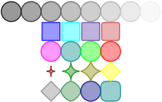
. Example ➛

Open the Javascript Console of your browser ( via menu, or shortcut F12 )
In the console, type Calc.colors.COLORNAME = "#RGB" , where RGB packs the R,G,B color components encoded in hexadecimal from 0 (min intensity ) to F (max intensity). E.g., Calc.colors.olive = "#880"
Variant: You can have more precision in the tint by encoding the colors as "#RRGGBB" , i.e. 2 digits for each color component from 00 (min intensity ) to FF (max intensity). E.g., Calc.colors.olive = "#808000"
You can then close the Javascript tab with the close button or F12.
Now, the color menu shows the extra colors !

Attention: the object colors are correctly saved, but at loading they will no longer appear as choice in the color menu.

➜ Conveniently packed by Andre Issa as a Color Picker plugin
. [ not working well on my ubuntu, though ]

[ To be continued ]

See also: secret geometry features , undocumented details

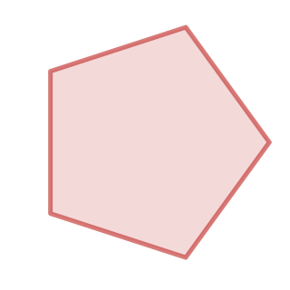
If you practice even a bit of Desmos Graph, you already know many way to draw curves (explicit, implicit, parametric, polar plot…) and to fill them (using inequalities). We also presented here how to draw series of curves and do more complex regions painting. With this we can already produce polygonal figures from equations:
polygons concentric polygons stars involved constructions
desmos-graph (23).png desmos-graph (24).png desmos-graph (25).png desmos-graph (26).png

But it is also possible to directly draw and manipulates shapes, and there are even undocumented features to do so.

At the base is the point: we already use them to draw parametrics ( X(t), Y(t) ), or to get visual sliders ( a, b ). This set point syntax. But there is a lot more you can do with points:

You can name them: A = (1,2), even for unknowns: X = (x,y)
Indeed they can even contain a list:
- X = [1,2,3] Y = [4,2,7] P = (X,Y)
  Or directly as T = ( [1,2,3], [4,2,7] )
  Or using an array. Example: Delaunay triangulation :
- This allows to define point sets:
  P = ( cos( 2Pi[0...N]/N ) , sin( 2Pi[0...N]/N ) )
Conversely, you can have list of points: L = [ (1,2), (3,5), (0,0) ]
That you can even translate and scale points and lists: (0,2) + .3 L
And mesure their offset: B - A
You can access point coordinates with P.x and P.y
You can draw polygons:
- polygon( A, B, C ),
  polygon( (1,1), (0,5), (5,3) ),
  polygon(P) with P defining a set above.
  The attributes button let you tune the look as for curves, with more options.
  - Note that polygons can be stored in variables and lists.
- Indeed you can also directly draw polylines or polygons when defining points set as P above: The attributes button let you join them with lines and tune exactly the same set of parameters.
  - trick: insert an impossible point ( e.g. (0,0/0) ) to create a line interruption.
- Arrays also let you display columns as point sets and tune attributes, allowing to draw points and join then with lines. Making them loop is not easy ( P[ join([1,...length(P)],[1])] ) , so it can be simple to duplicates the first point to the last position (explicitly, or by storing the duplicate values in some variables).
You can compute the distance between points (simples or sets):
distance(A,P)
You can get the midpoint(A,P)
Since version 1.6, you can add, substract, multiply points. E.g. (1-t)A + tB draws segment AB.
You can also use piecewise definition: C = { n=0: (1,2) , n=1: (0,7), (0,0) } . see example.
Example of application: drawing splines from point sets:
Alas we cannot directly solve or compare (e.g., A+X = B-X or midpoint( (0,0),(x,y)) = (5,5)).But we can do it on anything scalar:
- via their coordinates,
- we do can solve and compare with the distance operator:
  distance( (x,y), (0,0) ) <= 1 draws a filled circle.
  distance( (x,y), (0,0) ) = [0...N]/N draws a series of circles.
  distance( (x,y), (0,1) ) = distance( (x,y), (x,0) ) draws a parabola.
  More examples here.
  Attention: distance( (x,y), P ) = 1 with P as above would traces a series of circles, one around each points in the set, but distance( (x,y), P ) = [0...N]/N won't turn them into a double series (multiple circles around points): remember than arrays are synchronous in expressions, so each element of the array of radii will fit the corresponding element in the array of points.
Of course, you can also do geometry with points encoded as arrays, using points only for display and controls. Example here. Then,
- you can add, substract, weight points-as-arrays, cf 3D ellipse:
- dot product istotal(V1*V2),
- distance issqrt(total(V1²)),
- multiplication by matrix is [ total(V*[M00,M01]) , total(V*[M10,M11]) ],
- etc.
- ( drawing grids and vector fields: treated here ).
List comprehension now ease the drawing of meshes:
[ polygon( P(i,j),P(i+1,j),P(i,j+1),P(i+1,j+1) ) for i=[1...N-1],j=[1...N-1] ] with P(i,j) a function defining a point. Possibly P(i,j)=( X[i+Nj], Y[i+Nj] ) if you already have list of coordinates X[] and Y[].Use shape attributes to make it filled or wireframe.
With some effort, from all this you can even do meshes in 3D perspective:
see here, or a very complete examples here and there.

It's not uncommon to have either unexpected results or puzzling error messages in Desmos. Here are some classical examples and solutions.

Misleading functions

Desmos log means log10. Not to be confused with ln, that also be notedlog_e.
Desmos stdev means the statistical estimator, not to be confused with the real standard deviation of a set, noted stdevp. ( stdev = sqrt(N/(N-1))*stdevp ).

Misleading span of variables

There is no local variable. Sum_n prevents you to use n anywhere else again (and the error message will be puzzling)… but in other sums.
Lists are kind of vectors, but with common alignment for all expressions in your session. Don't expect to enlarge the combinatory by passing an extra vector where a constant was expected.

Ambiguous syntax

3 1/2 is considered as 3+1/2 rather than 3/2. Add parenthesis.
The syntax for tracing the locus where a variable or function equals something ( e.g., f(x) = 3 , or y₁ = a x₁² ) looks a lot like what you would do for defining it ( e.g. f(x) = x² , or y1 = S x + C y , x1 = C x - S y ) , and Desmos easily thinks it's a second definition of the same variable, which it allows… as long as its not used in another expression ( then you'll get a puzzling error message ).
→To avoid ambiguity, the left part must not look like a definition: rather use 3 = f(x) or f(x)+0 = 3 or +f(x) = 3 or (y₁) = a x₁²

Copy-pasting

From Desmos Graph to exterior, you will always get LaTeX form of equations. So Desmos can be used as a LaTeX editor, but you can't get simple text version.
From outside text to Desmos Graph: it works… but for operators like sqrt, |.|, {.}, sum …Indeed Desmos expect some LaTeX source, and just extend syntax to some text names like sin so that simple text expressions accidentally work. Conversely x_a = \sum{\sqrt{x}} works, or any complex LaTeX formula.But \{, that block the pasting.
New: some plugins now allow to manage that.

Out of conceptual space

Many limitations can be twisted, like drawing in 3D or emulating vector algebra. But some concepts remain definitively out of reach:

In fact all expressions are precomputed by Desmos. So don't expect to reproduce really evolving states, like dynamics simulation ( but with this hacky non-reliable hidden feature ) . Even recursivity won't work, for conditions are just functions like the others, rather than algorithmic structures.
There is no way you can get the inverse of a function, or find its zeros. But you can trace it.
Sometime you have to twist your mind to find a way to express a simple math relation. E.g. for AND, or worse, OR between conditions. Smart nesting of { } to obtain it is described here, section "restrictions". Sometime it's even more hairy, or impossible.
There are no true arrays or linear algebra: all tables are considered in sync and static. Sometime it might not compile, or worse, give an unexpected result due to that. A solution can be to explicit the target combinatory via a loop, or even a loop where L is a list.

Undocumented functions: (see more)

random(N)creates an array of N uniform random numbers in range 0..1.
random(N,s) provides a seed s allowing producing different sequences.
Note that it is not the standard seed allowing repeatable sequences, but just an extra shuffle.
Distributions: uniformdist(), normaldist(), poissondist(), binomialdist(), tdist() (student)
random(normaldist(...) , ... ) or normaldist(...).random(...) :
creates an array of random numbers with target distribution.
shuffle(L) shuffles list L (i.e., applies a random permutation).
So shuffle([1...N]) creates a random set on N unique values.
shuffle(L,s) provides an extra shuffle, as for random.

See example1 , example2.

Manually:

desmos-graph (21)

Of course, from this you can generates any random law, e.g., the Normal law:
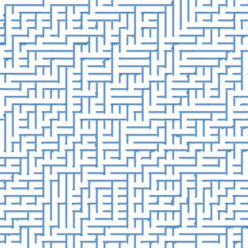
Just for fun, a (low quality) random maze equation:

How to Draw a Line Between Two Points on Desmos

Source: https://desmosgraphunofficial.wordpress.com/